PIVOT TABLE IN EXCEL
Introduction
A pivot table is a table which is used to store the summary of a certain data set in a condensed manner. The table consists of rows, columns, data fields, and pages. These components can be moved around and it helps the user to expand, isolate, sum, and group the particular data in real time. This table enables the user to view the differences in a very big set of information. It is very helpful in organizing a large amount of data in Microsoft Excel.
Working of the Table
A pivot table takes a user-specified data field and converts the header of each column into a data option which can be easily manipulated by the user. Columns containing data can be removed from, added to, or moved around the table quite easily. Here, user friendly and informative summaries can be created from long spreadsheets of raw data. The data can be summarized in various ways including frequencies and averages. Using the pivot table in excel has many benefits which are described below.
Easy to Use
An important advantage of pivot tables is that it is easy to use. You can easily summarize data by dragging the columns to different sections of the table. The columns can also be re-arranged as you wish with the click of a mouse.
An important advantage of pivot tables is that it is easy to use. You can easily summarize data by dragging the columns to different sections of the table. The columns can also be re-arranged as you wish with the click of a mouse.
Creating a Pivot Table
- Select any cell in the source data table.
- On the Ribbon, click the Insert tab.
- In the Tables group, click Recommended Pivot Tables.
- In the Recommended Pivot Tables window, scroll down the list, to see the suggested layouts.
- Click on the layout that you want to use, then click OK.
Pivot tables are one of Excel most powerful features. A pivot table allows you to extract the significance from a large, detailed data set.Our data set consists of 213 records and 6 fields. Order ID, Product, Category, Amount, Date and Country.

Insert a Pivot Table
Creating a Pivot Table
- Select any cell in the source data table.
- On the Ribbon, click the Insert tab.
- In the Tables group, click Recommended Pivot Tables.
- In the Recommended Pivot Tables window, scroll down the list, to see the suggested layouts.
- Click on the layout that you want to use, then click OK.
Pivot tables are one of Excel most powerful features. A pivot table allows you to extract the significance from a large, detailed data set.Our data set consists of 213 records and 6 fields. Order ID, Product, Category, Amount, Date and Country.

To insert a pivot table, execute the following steps.1. Click any single cell inside the data set.2. On the Insert tab, in the Tables group, click Pivot Table. The following dialog box appears. Excel automatically selects the data for you. The default location for a new pivot table is New Worksheet.3. Click OK.
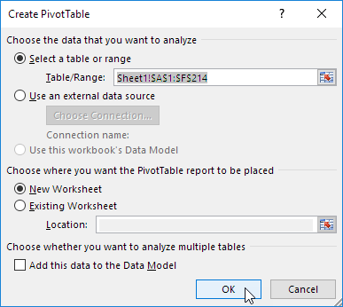
To insert a pivot table, execute the following steps.1. Click any single cell inside the data set.2. On the Insert tab, in the Tables group, click Pivot Table. The following dialog box appears. Excel automatically selects the data for you. The default location for a new pivot table is New Worksheet.3. Click OK.

Drag fields
The Pivot Table Fields pane appears. To get the total amount exported of each product, drag the following fields to the different areas.
1. Product field to the Rows area.
2. Amount field to the Values area.
3. Country field to the Filters area.
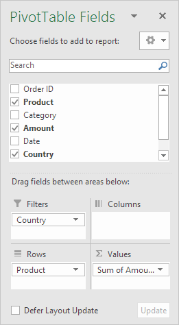
Below you can find the pivot table. Bananas are our main export product. That's how easy pivot tables can be!

Sort
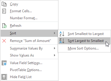
To get Banana at the top of the list, sort the pivot table.1. Click any cell inside the Sum of Amount column.2. Right click and click on Sort, Sort Largest to Smallest.
The Pivot Table Fields pane appears. To get the total amount exported of each product, drag the following fields to the different areas.
1. Product field to the Rows area.
2. Amount field to the Values area.
3. Country field to the Filters area.

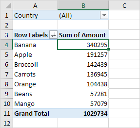
Below you can find the pivot table. Bananas are our main export product. That's how easy pivot tables can be!

Sort
To get Banana at the top of the list, sort the pivot table.1. Click any cell inside the Sum of Amount column.2. Right click and click on Sort, Sort Largest to Smallest.
Result.
Conclusion
In conclusion, our case is a good example of the added value Decision Support System, which can analyze great amounts of data, drill down on the data, identify the trends that helps manager to make a better decision and action plan in order to achieve the company's targets and goals.

Result.

Conclusion
In conclusion, our case is a good example of the added value Decision Support System, which can analyze great amounts of data, drill down on the data, identify the trends that helps manager to make a better decision and action plan in order to achieve the company's targets and goals.
Semma 👍🏻
ReplyDeleteNice
ReplyDelete